Python: Matplotlib-Graph plot

Rajesh

3 years ago

Python library for graph plotting: Matplotlib

Matplotlib is a plotting library for Python. It is used along with NumPy to provide an environment that is an effective open source alternative for MatLab.

It can also be used with graphics toolkits like PyQt and wxPython.
It was first written by John D. Hunter. Since 2012, Michael Droettboom is the principal developer.
Conventionally, the package is imported into the Python script by adding the following statement:

pip install matplotlib

import matplotlib.pyplot as plt

Graph Character description code

Plot Color: Character

Following formatting characters for color can be used.

Plot: X and Y- axis labels

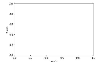
import matplotlib.pyplot as plt
plt.xlabel('x-axis')
plt.ylabel('Y axis')

Plot: Adding Title and Y- axis labels

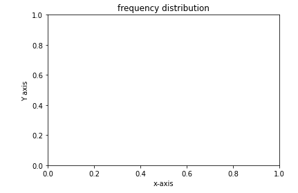
import matplotlib.pyplot as plt
plt.xlabel('x-axis')
plt.ylabel('Y axis')
plt.title('frequency distribution')

Plot: Grid

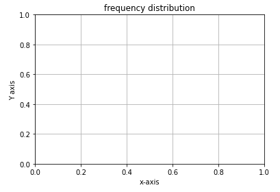
import matplotlib.pyplot as plt
plt.xlabel('x-axis') 
plt.ylabel('Y axis') 
plt.title('frequency distribution')  
plt.grid('true')

Line Graph

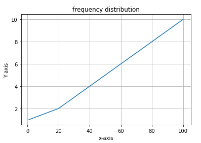
import matplotlib.pyplot as plt 
plt.xlabel('x-axis') 
plt.ylabel('Y axis') 

plt.title('frequency distribution') 
plt.grid('true')

x=(1,20,30,40,50,60,70,80,90,100)
y=(1,2,3,4,5,6,7,8,9,10)

plt.plot(x,y)

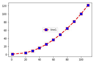
Line Graph: Marker & line style

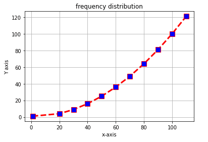
import matplotlib.pyplot as plt

x=(1,20,30,40,50,60,70,80,90,100,110)
y=(1,4,9,16,25,36,49,64,81,100,121)

plt.plot(x,y,c='red',linewidth=3, label='line1', linestyle='dashed' , marker='s', markerfacecolor='blue', markersize=10)

plt.xlabel('x-axis')
plt.ylabel('Y axis')

plt.title('frequency distribution')
plt.grid('true')
plt.show()

Line Graph: set X & Y Axis limit

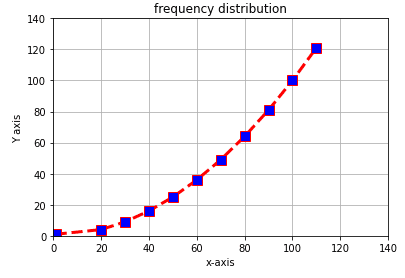
import matplotlib.pyplot as plt 

x=(1,20,30,40,50,60,70,80,90,100,110)
y=(1,4,9,16,25,36,49,64,81,100,121)

plt.plot(x,y,c='red',linewidth=3, label='line1', linestyle='dashed' , marker='s', markerfacecolor='blue', markersize=10)

plt.ylim(0,140)
plt.xlim(0,140)

plt.xlabel('x-axis')
plt.ylabel('Y axis')

plt.title('frequency distribution')
plt.grid('true')

plt.show()

Automatic Data generation & Graph plotting

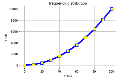
import numpy as np
import matplotlib.pyplot as plt

x=np.arange(0,101,10)
y=x**2

plt.plot(x,y,c='blue',linewidth=5, label='line1', linestyle='solid' , marker='s', markerfacecolor='yellow', markersize=10)

plt.xlabel('x-axis')
plt.ylabel('Y axis')

plt.title('frequency distribution')
plt.grid('true')

Plot: Two graphs on the same axis

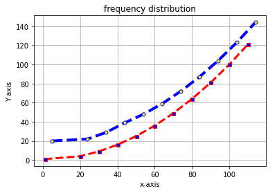
import matplotlib.pyplot as plt

x1=(1,20,30,40,50,60,70,80,90,100,110)
y1=(1,4,9,16,25,36,49,64,81,100,121)

x2=(5,24,34,44,54,64,74,84,94,104,114)
y2=(20,22,29,39,48,59,72,87,104,123,144)


plt.plot(x1,y1,c='red',linewidth=3, label='line1', linestyle='dashed' , marker='s', markerfacecolor='blue', markersize=5)

plt.plot(x2,y2,c='blue',linewidth=4, label='line2',linestyle='dashed', marker='o', markerfacecolor='yellow', markersize=5)

plt.xlabel('x-axis')
plt.ylabel('Y axis')
plt.title('frequency distribution')
plt.grid('true')

plt.show()

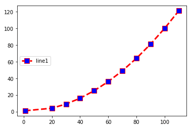
Graph: Legends location

Legend Location: Upper-right

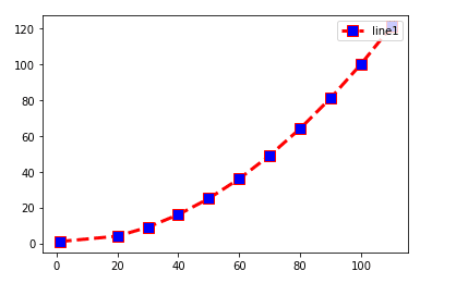
import matplotlib.pyplot as plt 

x =(1,20,30,40,50,60,70,80,90,100,110)
y=(1,4,9,16,25,36,49,64,81,100,121)

plt.plot(x,y,c='red',linewidth=3, label='line1', linestyle='dashed' , marker='s', markerfacecolor='blue', markersize=10)

plt.legend(loc='upper right')

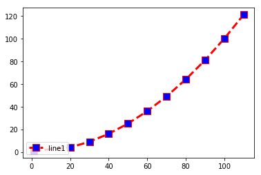
Legend Location: Upper-left

import matplotlib.pyplot as plt 

x =(1,20,30,40,50,60,70,80,90,100,110)
y=(1,4,9,16,25,36,49,64,81,100,121)

plt.plot(x,y,c='red',linewidth=3, label='line1', linestyle='dashed' , marker='s', markerfacecolor='blue', markersize=10)

plt.legend(loc='upper left')

Legend Location: Lower-left

import matplotlib.pyplot as plt 

x =(1,20,30,40,50,60,70,80,90,100,110)
y=(1,4,9,16,25,36,49,64,81,100,121)

plt.plot(x,y,c='red',linewidth=3, label='line1', linestyle='dashed' , marker='s', markerfacecolor='blue', markersize=10)

plt.legend(loc='lower left')

Legend Location: Lower-right

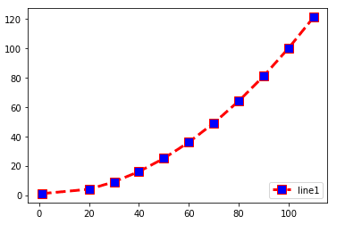
import matplotlib.pyplot as plt 

x =(1,20,30,40,50,60,70,80,90,100,110)
y=(1,4,9,16,25,36,49,64,81,100,121)

plt.plot(x,y,c='red',linewidth=3, label='line1', linestyle='dashed' , marker='s', markerfacecolor='blue', markersize=10)

plt.legend(loc='lower right')

Legend Location: Center-right

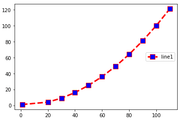
import matplotlib.pyplot as plt 

x =(1,20,30,40,50,60,70,80,90,100,110)
y=(1,4,9,16,25,36,49,64,81,100,121)

plt.plot(x,y,c='red',linewidth=3, label='line1', linestyle='dashed' , marker='s', markerfacecolor='blue', markersize=10)

plt.legend(loc='center right')

Legend Location: Center

import matplotlib.pyplot as plt 

x =(1,20,30,40,50,60,70,80,90,100,110)
y=(1,4,9,16,25,36,49,64,81,100,121)

plt.plot(x,y,c='red',linewidth=3, label='line1', linestyle='dashed' , marker='s', markerfacecolor='blue', markersize=10)

plt.legend(loc='center')

Legend Location: Center-left

import matplotlib.pyplot as plt 

x =(1,20,30,40,50,60,70,80,90,100,110)
y=(1,4,9,16,25,36,49,64,81,100,121)

plt.plot(x,y,c='red',linewidth=3, label='line1', linestyle='dashed' , marker='s', markerfacecolor='blue', markersize=10)

plt.legend(loc='center left')

Plot- Legend with maths equation

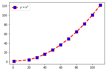
import matplotlib.pyplot as plt 

x=(1,20,30,40,50,60,70,80,90,100,110)
y=(1,4,9,16,25,36,49,64,81,100,121)

plt.plot(x,y,c='red',linewidth=3, label='line1', linestyle='dashed' , marker='s', markerfacecolor='blue', markersize=10)

plt.legend(loc='upper left')
plt.legend(['$ y=x^2

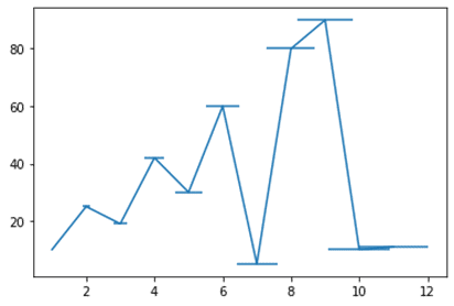
Bar graph -Vertical bar

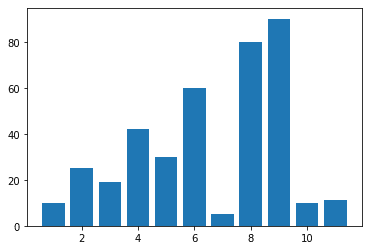
import matplotlib.pyplot as plt

y=(10,25,19,42,30,60,5,80,90,10,11)
x=(1,2,3,4,5,6,7,8,9,10,11)

plt.bar(x,y)
plt.show()

Bar graph – Horizontal bar

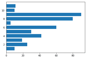
import matplotlib.pyplot as plt

y=(10,25,19,42,30,60,5,80,90,10,11)
x=(1,2,3,4,5,6,7,8,9,10,11)

plt.barh(x,y)
plt.show()

Bar Graph – with bar description

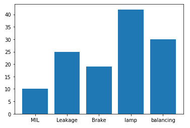
import matplotlib.pyplot as plt

x=('MIL','Leakage','Brake','lamp','balancing')
y=(10,25,19,42,30)

plt.bar(x,y)
plt.show()

Pie chart – Normal

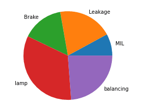
import matplotlib.pyplot as plt

x=('MIL','Leakage','Brake','lamp','balancing')
y=(10,25,19,42,30)

plt.pie(y, labels=x)
plt.show()

Pi chart- Exploded

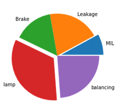
import matplotlib.pyplot as plt

x=('MIL','Leakage','Brake','lamp','balancing')
y=(10,25,19,42,30)

explode=(0.1,0,0,0.1,0)

plt.pie(y, labels=x, explode=explode)
plt.show()

Scatter Plot

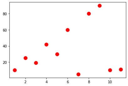
import matplotlib.pyplot as plt

y=(10,25,19,42,30,60,5,80,90,10,11)
x=(1,2,3,4,5,6,7,8,9,10,11)

plt.scatter(x,y,c='red',s=100)
plt.show()

Scatter Plot: Colour and Point size variation(within)

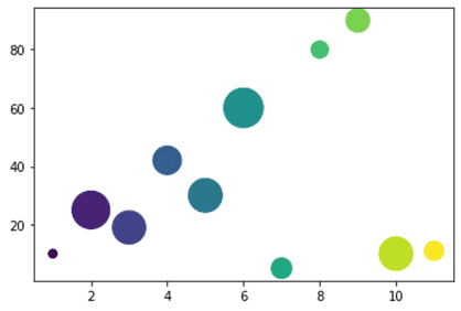
import matplotlib.pyplot as plt

y=(10,25,19,42,30,60,5,80,90,10,11)
x=(1,2,3,4,5,6,7,8,9,10,11)

col=np.arange(0,11,1)
pwidth=np.random.rand(11)**1*1000

plt.scatter(x,y, c=col, s=pwidth)
plt.show()

Scatter Plot: Color fading (alpha) effect

import matplotlib.pyplot as plt

y=(10,25,19,42,30,60,5,80,90,10,11)
x=(1,2,3,4,5,6,7,8,9,10,11)

col=np.arange(0,11,1)
pwidth=np.random.rand(11)**1*1000

plt.scatter(x,y, c=col, s=pwidth,alpha=0.3)
plt.show()

Histogram: Random number with a defined sigma value

import matplotlib.pyplot as plt

randomdata=np.random.normal(size=3000)*200
plt.hist(randomdata,bins=10)
plt.show()

Histogram: With increased Bins

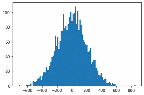
import matplotlib.pyplot as plt

randomdata=np.random.normal(size=3000)*200
plt.hist(randomdata,bins=100)

Histogram: With defined class width

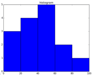
import matplotlib.pyplot as plt

a = np.array([22,87,5,43,56,73,55,54,11,20,51,5,79,31,27])
plt.hist(a, bins = [0,20,40,60,80,100])

plt.title("histogram")
plt.show()

Error plot ( X-error)

import matplotlib.pyplot as plt
import numpy as np
y=(10,25,19,42,30,60,5,80,90,10,11)
x=(1,2,3,4,5,6,7,8,9,10,11)

z=np.linspace(0,1,11)
plt.errorbar(x,y,xerr=z)

plt.show()

Error plot ( Y-error)

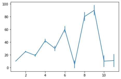
import matplotlib.pyplot as plt
plt.errorbar(x,y,yerr=z)

Sine graph

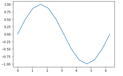
import numpy as np 
import matplotlib.pyplot as plt 

x=np.arange(0,2*np.pi+.1,np.pi/6)
y=np.sin(x)
z=np.linspace(0,2,13)

plt.plot(x,y)

Sine graph with Error plot

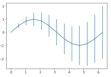
import numpy as np 
import matplotlib.pyplot as plt 

x =np.arange(0,2*np.pi+.1,np.pi/6)
y=np.sin(x)
z=np.linspace(0,2,13)

plt.errorbar(x,y,yerr=z)
plt.plot(x,y)

Error graph : Default Marker + Cap

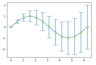
import numpy as np
import matplotlib.pyplot as plt

plt.errorbar(x,y,yerr=z,marker='s',mfc='yellow' , capsize=10 )

Error graph : Marker(bigger) + Cap(bigger)

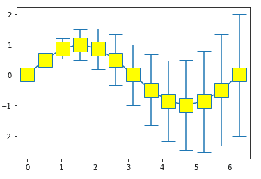
import numpy as np
import matplotlib.pyplot as plt

plt.errorbar(x,y,yerr=z,marker='s',mfc='yellow' , markersize=20,capsize=10 )

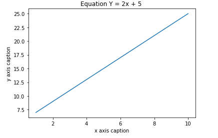
**Plot : Math equation (Y = mx + c)**

import numpy as np
import matplotlib.pyplot as plt

x = np.arange(1,11)
y = 2 * x + 5

plt.title("Equation Y = 2x + 5")
plt.xlabel("x axis caption")
plt.ylabel("y axis caption")

plt.plot(x,y)
plt.show()

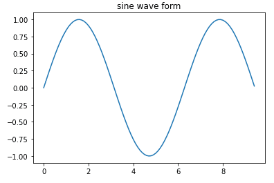
Plot- Sine wave

import numpy as np
import matplotlib.pyplot as plt

x = np.arange(0, 3 * np.pi, 0.1)
y = np.sin(x)

plt.title("sine wave form")
plt.plot(x, y)

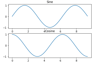
Two graphs: Vertical Stacking

import numpy as np
import matplotlib.pyplot as plt

# Compute the x and y coordinates for points on sine and cosine curves

x = np.arange(0, 3 * np.pi, 0.1)
y_sin = np.sin(x)
y_cos = np.cos(x)

# Set up a subplot grid that has height 2 and width 1,

# and set the first such subplot as active.

plt.subplot(2, 1, 1)

# Make the first plot

plt.plot(x, y_sin)
plt.title('Sine')

# Set the second subplot as active, and make the second plot.

plt.subplot(2, 1, 2)

plt.plot(x, y_cos)
plt.title('Cosine')

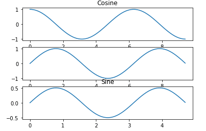
Three Graphs: Vertical Stacking

import numpy as np
import matplotlib.pyplot as plt

x = np.arange(0, 3 * np.pi, 0.1)
y_sin = np.sin(x)
y_cos = np.cos(x)

plt.subplot(3, 1, 1)
plt.plot(x, y_cos)

plt.title('Cosine')

plt.subplot(3, 1, 2)
plt.plot(x, y_sin)

plt.subplot(3, 1,3 )
plt.plot(x/2, y_sin/2)

plt.title('Sine')
plt.show()

Three Graphs: Vertical Stacking

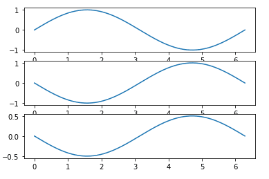
import numpy as np
import matplotlib.pyplot as plt

fig, A = plt.subplots(3)

x = np.linspace(0, 2 * np.pi, 400)
y=np.sin(x)

A[0].plot(x,y)
A[1].plot(x,-y)
A[2].plot(x,-y/2)

Three Graphs: Horizontal Stacking

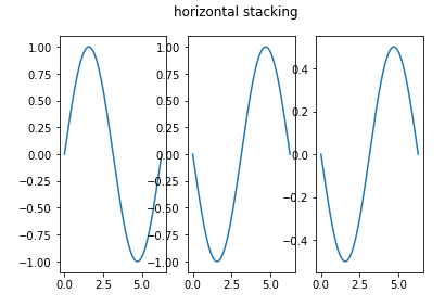
import matplotlib.pyplot as plt
import numpy as np

fig,(A1,A2,A3) = plt.subplots(1,3)

x = np.linspace(0, 2 * np.pi, 400)
y=np.sin(x)
A1.plot(x,y)
A2.plot(x,-y)
A3.plot(x,-y/2)

fig.suptitle('horizontal stacking')

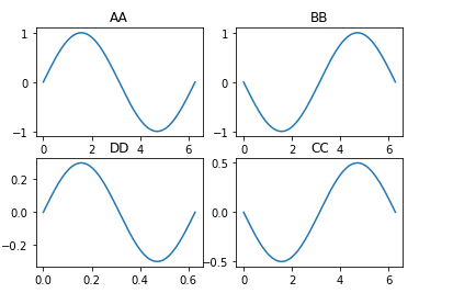
Four graphs Horizontal & Vertical Stacking

import matplotlib.pyplot as plt
import numpy as np

fig, A = plt.subplots(2,2)

x = np.linspace(0, 2 * np.pi, 400)
y=np.sin(x)

A[0,0].plot(x,y)
A[0,0].set_title('AA')
A[0,1].plot(x,-y)
A[0,1].set_title('BB')
A[1,1].plot(x,-y/2)
A[1,1].set_title('CC')
A[1,0].plot(x/10,y*0.3)
A[1,0].set_title('DD')

Graph: Horizontal & Vertical Stacking in Multi-Color

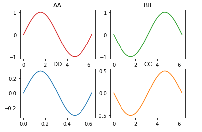
import matplotlib.pyplot as plt
import numpy as np

fig, A = plt.subplots(2,2)

x = np.linspace(0, 2 * np.pi, 400)
y=np.sin(x)

A[0,0].plot(x,y, 'tab:red')
A[0,0].set_title('AA')
A[0,1].plot(x,-y, 'tab:green')
A[0,1].set_title('BB')
A[1,1].plot(x,-y/2, 'tab:orange')
A[1,1].set_title('CC')
A[1,0].plot(x/10,y*0.3)
A[1,0].set_title('DD')

Four Graphs: Horizontal + Vertical Stacking (X-axis equal span, all graphs)

import matplotlib.pyplot as plt
import numpy as np

fig, A = plt.subplots(2,2, sharex=True )

x = np.linspace(0, 2 * np.pi, 400)

y=np.sin(x)
A[0,0].plot(x,y)
A[0,0].set_title('AA')
A[0,1].plot(x,-y)
A[0,1].set_title('BB')
A[1,1].plot(x,-y/2)
A[1,1].set_title('CC')
A[1,0].plot(x/10,y*0.3)
A[1,0].set_title('DD')

Four Graphs: Horizontal & Vertical Stacking (X & Y equal span, all graphs)

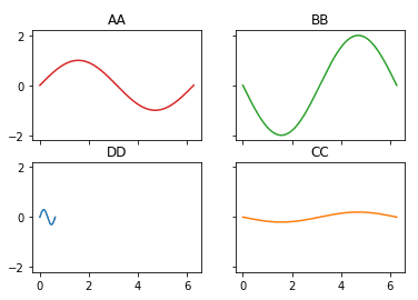
import matplotlib.pyplot as plt
import numpy as np

fig, A = plt.subplots(2,2,sharex=True , sharey=True)

x = np.linspace(0, 2 * np.pi, 400)
y=np.sin(x)

A[0,0].plot(x,y, 'tab:red')
A[0,0].set_title('AA')
A[0,1].plot(x,-2*y, 'tab:green')
A[0,1].set_title('BB')
A[1,1].plot(x,-y/5, 'tab:orange')
A[1,1].set_title('CC')
A[1,0].plot(x/10,y*0.3)
A[1,0].set_title('DD')

Two graphs with a common X-axis

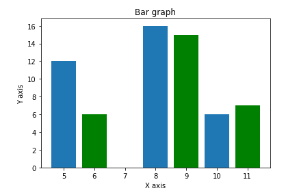
import matplotlib.pyplot as plt
import numpy as np

x = [5,8,10]
y = [12,16,6]
x2 = [6,9,11]
y2 = [6,15,7]

plt.bar(x, y, align = 'center')
plt.bar(x2, y2, color = 'g', align = 'center')

plt.title('Bar graph')
plt.ylabel('Y axis')
plt.xlabel('X axis')

Two graphs with a common Y-axis

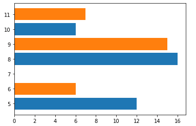
import matplotlib.pyplot as plt
import numpy as np

x1 = [5,8,10]
y1 = [12,16,6]
x2 =[6,9,11]
y2 =[6,15,7]

plt.barh(x1,y1)
plt.barh(x2,y2)

plt.show()

The package is available in binary distribution as well as in the source code form on