
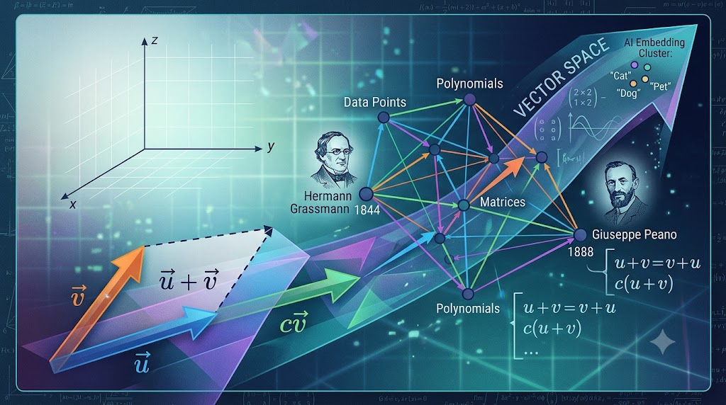
1. Historical Background & Origins
Long before “vector spaces” existed as a formal mathematical concept, natural philosophers and physicists were struggling to quantify entities that could not be characterized by a single numerical value. Quantities such as velocity, acceleration, and force demanded both a magnitude and a direction.
The Parallelogram Law
In classical mechanics, Isaac Newton and Daniel Bernoulli formalized the insight that two physical forces acting simultaneously on an object combine geometrically. The resultant force corresponds to the diagonal of a parallelogram formed by the two individual force arrows.
With René Descartes’ invention of analytic geometry, space was equipped with numerical axes (x, y, z). Geometry was transformed into algebra, allowing lines and planes to be described using linear equations.
In the mid-19th century, Sir William Rowan Hamilton introduced quaternions—four-dimensional hypercomplex numbers—to model rotations and directions in 3D physical space. Hamilton coined the term “vector” (derived from the Latin vehere, meaning “to carry”) to describe the imaginary part of a quaternion. However, mathematicians soon realized that vectors could be detached from quaternions and physical spatial restrictions altogether.
Grassmann’s Breakthrough (1844)
“Why should geometric thinking be restricted to three dimensions simply because our physical perception is three-dimensional?”
In his masterpiece Die Ausdehnungslehre (The Theory of Extension), Hermann Grassmann formulated an algebraic system where points, lines, and volumes were represented as elements of arbitrary n-dimensional spaces. Though largely ignored during his lifetime due to its dense philosophical prose, Grassmann’s work laid the true conceptual foundation for modern linear algebra.
In 1888, Italian mathematician Giuseppe Peano formally synthesized Grassmann’s work in his text Calcolo Geometrico. Peano stripped vectors of their geometric ties, providing the first modern, axiomatic definition of a linear system based entirely on operational rules rather than spatial interpretation.
2. Formal Definition & The Axioms of a Vector Space
A vector space (or linear space) over a field F (such as the field of real numbers ℝ or complex numbers ℂ) is a non-empty set V equipped with two operational maps:
For V to be a vector space, these operations must satisfy the following eight axioms for all vectors u, v, w ∈ V and all scalars a, b ∈ F:
The 8 Fundamental Peano Axioms
3. Fundamental Properties & Core Theorems
From the foundational Peano axioms, several core structural properties can be rigorously proved. These properties guarantee algebraic stability across all valid vector spaces.
Theorem 3.1: Uniqueness of Zero and Inverses
In any vector space V, the zero vector 0 is unique. Furthermore, for every vector v ∈ V, its additive inverse −v is strictly unique.
Theorem 3.2: Multiplication by Zero Scalar
For any vector v ∈ V, multiplying by the field scalar 0 ∈ F yields the zero vector: 0 · v = 0.
Theorem 3.3: Cancellation Law
If u, v, w ∈ V and u + w = v + w, then u = v.
Theorem 3.4: Subspace Criterion
A non-empty subset W ⊆ V is a subspace of V if and only if it is closed under linear combinations: ∀ u, v ∈ W, ∀ a, b ∈ F ⟹ (au + bv) ∈ W.
4. Classic & Diverse Examples
Because vector spaces are defined purely by operational axioms, objects of widely different mathematical natures—tuples, matrices, polynomials, and continuous functions—all form valid vector spaces.
| Vector Space V | Element Structure | Field F | Dimension |
|---|---|---|---|
| Coordinate Space ℝⁿ | n-tuples of real numbers (x₁, …, xₙ) | ℝ | n |
| Polynomial Space Pₙ(x) | Polynomials of degree ≤ n | ℝ or ℂ | n + 1 |
| Matrix Space Mₘ,ₙ(ℝ) | m × n matrices with real entries | ℝ | m × n |
| Function Space C[a,b] | Continuous functions f : [a,b] → ℝ | ℝ | Infinite (∞) |
| Sequence Space ℓ² | Square-summable sequences (xₖ) | ℂ | Infinite (∞) |
5. Modern Vector Space Theory & High-Dimensional Applications
In the 20th century, David Hilbert and Stefan Banach generalized vector spaces to infinite-dimensional topological structures, creating the field of functional analysis:
- Banach Spaces: Complete normed vector spaces allowing rigorous limits and calculus on functions.
- Hilbert Spaces: Vector spaces equipped with an inner product that defines angles and orthogonality in infinite dimensions—forming the mathematical foundation of Quantum Mechanics.
Vector Spaces in Modern Artificial Intelligence & Signal Processing
Modern Machine Learning algorithms process complex real-world data by mapping entities into high-dimensional vector spaces (Embedding Spaces):